Symmetries in our fractal world 

(Version vom 11.11.2015) 

1 Introduction 

The answer to the origin of our world or the universe can at the earliest be explained by the physics with all the theories and formulas. Many physical phenomena can be explained by simple linear equations and many others can be explained by cubic or square root equations. It seems that our universe is a universe of symmetries and patterns. But on the other side the chaos is also part of our universe. This part cannot be explained directly. These two components belongs always together in galaxies, atoms, weather-phenomena or human society-structures. Can it even be that such fractal structures are part of our human mind or even the mathematics of our physics. In the following text the symmetries the similarities and the links between of the great two theories of physics are described. The theory of relativity was developed for extreme big but nearly static structures and the quantum mechanics for extreme small but nearly infinite fast processes. The unification of these "last" theories would explain all details of our extreme complex world. This means that the unification is even infinite complex if every possible simplification has been applied. How can we explain our complex and fractal world in a "nearly" understandable way. Unfortunately we cannot explain everything but only special views. 

2. Main part 

2.1 Interference of stationary waves in moving inertial systems 

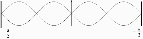
We start width known basics. First we consider a classical 3-dimensional Euclidean space. In this system S1 defines a wave oscillating between two reflectors having a distance a. The wavelength should be exact be length to establish a stationary wave. 

Fig. 1   

Now we imagine that we move with the reflectors in a inertial system S2 width a constant velocity v to the right. The waves propagation width the velocity c should be the same as in the previous example. We define the inertial system S1.

Fig. 2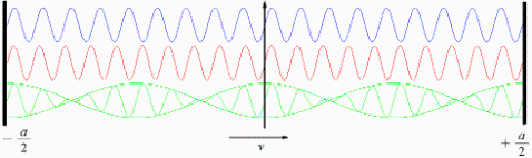   

The red and blue wave in fig. 2 shows a waves running to the left and right. For the inertial system S2 it should be clear that the propagation velocity for the red wave is c-v and for the blue wave c+v. We cannot guarantee a stationary wave anymore. By mirroring the wave on the reflectors the frequency is changing. The resulting "green" wave shows that for special "quantum"-velocities stationary waves can still develop. We calculate some relations: 

[Eq. 1]    duration for a wave front in the inertial system S1 for the distance a 

[Eq. 2]    duration for a wave front running to the right in inertial system S2 for the distance a 

[Eq. 3]    duration for a wave front running to the left in inertial system S2 for the distance a 

We calculate durations for a complete way forth and back in S1 and S2. 

[Eq. 4]    duration for a wave front forth and back in S1 

[Eq. 5]    duration for a wave front forth and back in S2 

We equate the durations for a complete way forth and back (constant duration). Width we get a time-dilation-factor / : 

[Eq. 6]   

[Eq. 6]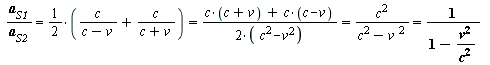   

We also can equal the track (constant length) and we get a time dilatation factor / : 

[Eq. 7]      und    

[Eq. 7]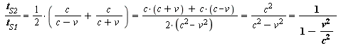   

Theoretical the limit for a constant time as the same as the limit for a constant length can make sense. In nature extremes are rare. That's why we can assume that a intermediate state will establish. We consider now some other limits: 

- Is the amount of wave-mountains high, for many velocities a stationary wave is possible. In extreme case for a infinity high frequency this is possible for every velocity (see also section 3.2).  

- On the other side if there is only one wave-mountain only for the velocity v=0 a stationary wave is possible.
 

2.2 The definition of a time in 3-dimensional space 

We want to consider now a different view. A wave-front of a spherical wave should expand in an inertial system S1 (Euclidean space). The expansion-velocity c is constant in all 3 space-directions. To illustrate this the diagram in Fig. 3. shows a surfer who is surfing width constant velocity in the direction of the y-axis in time. The x-axis describes a space-dimension. 

Fig. 3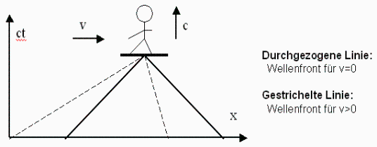   

The wave front of the "bow wave" expands in positive and negative x-direction width the velocity c. Simultaneously the surfer is moving in direction y in the time. We get an expansion cone (shown in Fig 3 as continuous line). Is the moving velocity in time exact the same as the wave-velocity the angle between the wave-fronts is exact 90 degree. Now the surfer should also move additional to the time also in direction of the x-axis. The wave front is shown in Fig 3 as broken line. If we expect that the angle should still be 90 degree the velocity in time must be the same the wave velocity. But now not in direction y-axis but a little bit to the side width a 45° angle to the wave front. Mathematically we can describe this as rotation. 

But for a absolute time-reference a constant y-velocity is expected. For a 90 degree angle between the wave fronts we can scale the y-axis width a factor (dilatation of the length). We measure the durations of the wave front in an stationary and a distance a in the moving inertial system. We get the same equations 1-3 we also got with our stationary wave. 

[see eq. 1]    for a wave front in a not moving system S1 (v = 0)  

[see eq. 2]    for a rrigth moving wave front in a moving system S2 (v > 0)  

[see eq. 3]    for a left moving wave front in a moving system S2 (v > 0) 

In our real world the velocity of light is in all inertial systems constant. That's why the arrival of a light wave defines the existing of an event. On the right side the wave arrives in system S2 later than in S1. That's why our clock is in relation to S1 a little bit faster. Width this definition of a temporal distortion we can bend our world in such a way that we get the wanted result of a constant velocity of light in all inertial systems. In our imagination not only the wave "flows" but also the time from a point into the surrounding space. 

Now we assume that the surfer moves into the opposite direction -v. We have to mirror the diagram around the x-axis. Using a Interferometer like the one Michelson and Morley used exact the same happens on every moment because the light beam moves into opposite directions. To explain in another way we define a "forward wave". This is a wave flowing always away from the viewer. The "backward wave" moves inverted back to the viewer. But how can we combine theses two pictures? The solution is a something like a zigzag-movement. At every moment the surfer moves a little bit to the left and afterwards the same distance to the right. By hacking the waves we get a solution for the dilatation factors (for time and space). And by viewing it from a distance we get the impression of a smooth movement. That's enough for the moment. 

2.3 Space-space-loops and space-time-loops 

We consider now the equation of the wave expansion in space width a radius r. The relation between space-dimensions x,y,z and the time is shown in eq. 8.  

[Eq. 8]      bzw.     

The basis for a dimension is always the definition of a linear independence to all the other dimensions. Sorry, but that's correct for the 3-dimensional space but not for a 4-dimensional space-time. We can claim that the z-dimension is the result of a new "3-dimensional" x-y-time-world is. We get a world width a linear independent time-dimension. 

[Eq. 9]     bzw.     

By dividing the formula in a different way we get something like a function for a circle. A x-y-loop is equal to a the z-time-loop or in another way the z-time-loop is equal to a x-y-loop: 

[Eq. 10]   

[Eq. 11]   

There are 6 possible combination: 

 x-time-loop    y-time-loop     z-time-loop  

 x-y-loop       x-z-loop        y-z-loop 

Using the Euler formula we can show that rotating a system can be nicely written as a complex exponential function. The wave function is a function of space and time. We assume that x is not a space-vector but only a dimension. Additional constants are the amplitude A, the wavenumber k and the frequency ω. By dividing the space and time we see that half of the possible loops spread a space. The division between room and space is chosen by random (link to the 4d-space-time). 

2.4 Linear combinations between inertial systems 

Considering now two inertial systems S1 and S2 in a Euclidean space. The length of the system S2 should be compressed by a factor On the other way around the inertial system S1 has to be stretched by the same factor or in other words it is compressed by the inverted factor By multiplying both factors together we get always 1. This is valid for all linear systems like our 3 dimensions and the time. 

[Eq. 12]   

[Eq. 13]   

2.5 The constant speed of light 

Now we add the fundamental physical condition of the constancy of the speed of light in all inertial systems. Even in our 3d-space we can change the inertial system S2 and get a correct and constant wave velocity if we slow down the time by a factor f and at the same time expand the 3-dimensional-space width the factor f. This is the direct solution for the formula that a distance a divided by the used time t is the (wave) velocity c. 

[Eq. 14]    

We can scale linear systems by a any factor we want. Further more it has to be possible that we can scale a random initial system in time and space such a way that we get a unified wave velocity. That's why c is only a transformation-factor between the physical quantities space and time. Everything else is relative, scaleable and symmetric. 

[Eq. 15]    

2.6 The interference of waves 

The quantum theory suggests that the reflectors of our stationary wave (section 2.1) are being replaced by another stationary wave. The stationary wave is its own mirror and interfering width itself. Further more the wave is its own propagation medium. We assume that we are part of a new initial system S0. Relating to this system S0 the system S1 is flowing width the same velocity v* to the left as the system S2 is flowing to the right. Referring to S0 the systems S1 and S2 should be symmetric to each other except the other moving directions. 

Fig. 4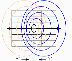   

Now we are trying to interfere in system S0 systems from section 2.1. In a very small point in the wave origin it should be possible. To compare relating systems we expect for both systems the exact same scale-factors in space and time. We expect with eq. 12 that is correct for space and time. With eq. 13 we must accept . Following . This is a direct conflict because eq. 6 and 7 are expecting . 

To satisfy all the criteria we have to accept that the factor / and the inverted factor / can only exist if we assume a additional (space-)dimension. Something similar can be applied for the time-scaling-factors / and / The additional dimension can be also the each other dimension. That's why we need only one additional dimension. Referring to fig. 4 we imagine that the face is rotating into and out the screen. For us only the distortion is visible. We go back to the wave function from Section 2.3. We are rotating the phase-angle ϕ twice: 

[Eq. 16]   

In eq. 16 the phase-angle was extracted out of the exponent and written as Product. We imagine the are distortion-factors and we expect that the new factors a/a' and t'/t referring to S0 and S1 or S0 and S2 can be multiplied together in the same manner as the Both rotations together are creating the distortion-factor between S1 and S2. Now we make sure that the distortion-factors are comparable. From our point of view we are rotating in case 1 only in one direction. In case 2 we are rotating to both sides. Referring to the viewer all rotations and scaling are the same. We can now be sure that our calculation is correct and we have no recursions in the dependencies. 

Case 1: point of view is S2. Distortion-factors are / und / referring to system S1. 

       = point of view is S1. Distortion-factors are / und / referring to system S2. 

Case 2: point of view is S0. Distortion-factors are a/a' and t'/t bezüglich S1 und bezüglich S2. 

         The factors referring S1 and S2 should be the same because of the same velocities v*. 

         The rotation-direction from S1 and S2 referring to S0 should be counter rotating. 

Following: 

[Eq. 17]   und    

We set eq. 6 and 7 into eq. 17: 

[Eq. 18]    (Gl. 6 und 7) 

By inverting the formula we get a stretching-factor and a compressing-factor. Both factors make sense but for us one factor is more familiar: 

[Eq. 19] 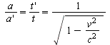    (the Lorentz factor)  

The factors for space and time are the same. By having a balance between space and time this is exact the value we have expected. 

2.7 Scaling of the size 

Now we want get a logic explanation for the balance-process from section 2.6. The fig 4 shows that the left-movement cannot be combined directly width the right-movement because the waves are mirrored. That's why the waves drift apart. The only point that is comparable is the point at the origin of the wave. The calculations are valid only for a wave width a infinity small radius. This is in conflict width imagination that in fig 2 only for special "quanted" velocities a stationary wave is possible. To get a stationary wave for all possible velocities we need a infinity large amount of waves. This is in conflict to the picture of a infinity small spherical wave. It seems that the Lorentz transformation is valid only if big wave-structures and small wave-structures are interfering together. 

The theory of relativity can ignore a absolute inertial system like a ether using the relativistic principle. The described principle can confirm this by image that the waves propagation medium is once again the same wave. In addition to this the principle can ignore a absolute size. Only the relation between length and time is important ad even this can be scaled by the velocity. By examine some known structures like quarks, protons, atoms, planets, stars, galaxies, galaxy clusters, universes it doesn't make sense that the quark is the smallest existing and the universe the biggest existing. In physics it will be extremely hard to discover greater or smaller structures because of the measuring limits. As the wave-particle-dualism can explain the same matter from two different perspectives of view, in the same manner also the size can be interpreted on different ways. Presumably it is even undecidable if our universe is expanding or not. The red-shift of vast distant objects can be interpreted as "bending" of the edge of our universe-bubble in an even greater multiversum. 

2.8 Definition of energy and energy-density 

Regarding a stationary wave in fig. 5. In all 3 diagrams a line from the right reflector to the left reflector has always the same length for all frequencies. This is not only correct for a triangle but always if a wave is scaled (space direction x and amplitude A) by a factor n and afterwards inserted n times between the reflectors. A explanation for this is the scalar product where by scaling all components by a factor n also the vector itself is scaled by the factor n. 

Fig. 5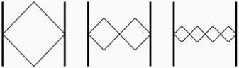   

Considering a special sinus wave width a gradient of 1 at the zero-crossing: 

[Eq. 20]      for example at x=0     

In fig 5 the system energy is always the same because rubber-bands would be stretched the same in all cases (see also section 3.3). But the energy density w in the compressed system is in relation to the not scaled system by a factor n greater. That's because of the scaling of the amplitude by the factor n. In the same space is room for n-times more energy. 

Do we compare the scaling factor n for a distortion (see eq. 6) and a self-interfering wave width the Lorentz factor (see eq. 19). Because the Lorentz factor from section 2.6 can be interpreted as a rotation in a multi-dimensional space, the velocity width a special value 1/ is used. The value is equivalent to a rotation of π/4 or 45° and is a important symmetry.  

[Eq. 21]    

If we set in equation 6 and 19 we get: 

[mit Gl. 6]   

[mit Gl. 19]   

A quadratic function in a Euclidean space is translated to a linear function if the wave is its own propagation medium. If in a Euclidean space we have to rotated around x-axis and y-axis. On the other side we only need to scaled by one axis in a self interfering system. The second rotation is the space-time. From an Euclidean space energy in an oscillating system (see section 3.3) is translated to or depending if the length (rotation around y-axis) or the amplitude (rotation around x-axis) is scaled. If we demand a constant amplitude then we get a reference to Planck's quantum of action: 

[Eq. 22]      Reference to Planck's quantum of action 

In fig. 5 a sinus wave has been expressed by simple squares. We can describe and understand fractal patterns only by simplifying systems (Fig. 6). 

Fig. 6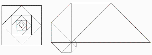   

2.9 Bended path 

In an Euclidean space a object should bonded on an circular path. It should be rotating around the centre width a constant velocity v. The path that is needed for a angle α is proportional to the radius r. This is the result from the linear dependency of the circumference U and the radius r (). We need for a smaller radius r and the same velocity a linear greater force to hold the object on the circular path. The force should be expressed by a energy density gradient. 

[Eq. 23]   

Fig. 7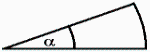   

This should be correct also for waves width a constant velocity v=c. To hold the wave on its path we imaging that the wave is refracted in a lens. The energy density potential has to be the same anti proportional form as in our first example. All waves that a caught in such a loop we interpret as mass. Has the mass in a disc a 1/r - distribution then all objects are rotating width the same angle velocity.

Relativistic view of the big:  

A stationary wave (see section 2.1) can exist also for a motioning systems if space and time is distorted. In the furthest limit for the greatest velocity v=c the observed space after eq. 7 and eq. 7 has to be distorted endless (pole on the y-axis in fig. 8). 

Quantum mechanic view of the small: 

On the other side a space has to be stretched endless if a light wave on the border of the potential pot stands still with the velocity v=0. This is the moment when the oscillating point is changing the moving direction. For a viewer the velocity v=c is valid. (pole on the x-axis in the fig. 8.)  

The model of balance: 

- Relativistic a object rotates only loss-free around a mass if the mass is infinity great. In all other cases particles in form of gravitational waves were emitted. Only a 1/r potential creates a balance (mass distribution in maximal chaotic galaxies). 

- In quantum mechanics bosons likes to the same state. The result is that the structure is not flowing apart. The nature of fermions is responsible for the quantum mechanical states and the reason why the wave is not falling into the centre. Like in Nature all states has to be occupied. 

Fig. 8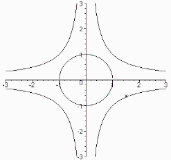   

Is the theory of relativity is valid for a limit of the great and the quantum mechanics as limit for the small? Energy overlaps in it's most compact form to something like the coulomb potential. For greater gradients the wave breaks and flows apart. A area width a small gradient is filled width new particles immediate. For the limit for a infinite high waves frequency a infinity high energy is the result. In real energy-potentials the energy is limited because the continual interactions of the inner particles. Because of the "not ideal" coulomb-potential it's possible that the potential-field creates new structures. For example a electron is created by the potential pot of the proton. 

Because of the stationary wave the outer border of the coulomb potential is not smooth but jagged somehow. Usually such oscillating movements are stimulating other oscillations. If something is moving then always by a whole wavelength. Presumably all particles in our universe have a common resonance frequency. The theory of a control-field can possibly explain the wave-particle-dualism or bells inequations. Can we describe our world from the quark to the universe as a infinite complex and knotted space? Is the imagination of fractal spirals the most simple view of our universe? Our universe has more symmetries than thought for example the symmetry of a sphere surface. One thing is important - nothing is absolute. Even the gravitation constant and the velocity of light can only exist in connection to the space and the viewer. The gravitation constant can be explained as "remain"-energy that is left over after all particle-interactions. In the opposite the velocity of light would be in a infinity dense medium after Einstein infinite small (infinite small time). At the border of our universe the velocity of light has to be infinite fast. Or in other words must the space be spread endless there. Space and time are creating each other and generate our universe. All is relative, invertable and fractal but what happens if mankind accepts that they are also part of the system. 

Fig. 9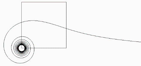   

3 Mathematic appendency 

3.1 Derivation of a stationary wave 

It can be shown that 2 flowing waves width a oppsite direction can interfere to a stationary wave. 

[Eq. 30]  


 

The new formed interfered wave has a temporal factor that is independent from x. Thats because the phase stays constant over time. 

3.2 The derivation of high frequent interering waves in a moved system 

Two in opposite direction running waves can be interfered to a stationary wave. The wave should be shifted by a phase angle ϕ. This condition has to be valid if stationary waves can be formed in a moving potentional pot. The staionary wave should have exact the same form as same as the same frequecy and wave length as the origin wave. 

[Eq. 31]  

 

If the phase displacement is excact a multiple of the wave length then the phase displacement can be ignored. For very large frequencies ω also the n would bs very large. The step to the next natural number n+1 would be very small in relation. The possibility that for a stationary wave can build a stationary wave increases for higher frequncies. At large frequencies is this proportional to the frequency. 

3.3 Derivation of not damped harmonic oscilations 

We consider a not undamped harmonic wave. The entire energy is result of the potential energy and the kinetic energy . 

[Eq. 32]   

 k = wavenumber
 m = mass
 v = velocity
 y = amplitue 

At the waves zero crossing we have und . Additional to this the velocity at the zero crossing is maximal . Width follows: 

[Eq. 33]      or     

The energy is squared proportional to the amplitude and to the frequency. Both are antiproportional to each other at constant energy. 

4. Open questions 

- Why does in a large atom every proton has its own electron? Where does such resonance patterns come from? Has the electron a spin because of the structure of the quarks?  

- How many symmetries has a atomic particle? What's the difference between particles and antiparticles? Fermions and bosons? Right handed and left handed particles (for examples neutrinos)? Why dos neutron decays into protons, electrons and antineutrinos? Because of the definition? 

- Can a black hole be interpreted as a atomic particle? Can our universe can be interpreted as atomic particle? This could explain the redshift of very distant objects without the need of a expansion of the universe. Is this a explanation for the dark matter? 

- Exact the half all loop-possibilities (out of section 2.3) are spanning a space. Is the energy in our universe divided to one half to the space and to one half to the space? Has the first symmetry break divided our universe into space and time? Can we equal symmetries and information? 

- Why are all protons are the same? Why is the mass exact the same? Gets everything in the very small and in the very big more and more the same and more symmetric. Can we recognize some symmetries better? Very fast processes can be analyzed in a very small space because enough information can be gathered to localize symmetries. Are the processes extreme slow and almost static then a large space has to be observed to discover patterns. This in a formula could be the quantum mechanics and the theory of relativity? 

5. Literature 

Dr. rer.nat. Theo Mayer-Kuckuk: Atomphysik Eine Einführung 2. Auflage 1980 

Dr. rer.nat. Theo Mayer-Kuckuk: Kernphysik Eine Einführung. 6. Auflage 1994 

Albert Einstein: Über die spezielle und die allgemeine Relativitätstheorie. 21. Auflage 1969 

Wolfgang Pauli: Relativitätstheorie. 2000 (Originalausgabe 1921 erschienen in der Encyklopädie der Mathematischen Wissenschaften Bd. V) 

Joseph Polchinski: WHAT IS STRING THEORY? 1994 

Frank Close: Das Nichts verstehen. Originalausgabe: The Void. 2007  

Kuchling: Taschenbuch der Physik. 15. Auflage 1995